1. Introduction
Understanding the functional role and evolutionary relationships of proteins is key to answering many important biological and biomedical questions. Because the function of a protein is determined by its structure and because structural properties are usually conserved throughout evolution, such problems can be better approached if proteins are compared based on their representations as three-dimensional structures rather than as sequences. Databases, such as SCOP (Structural Classification of Proteins) [
1] and CATH [
2], have been built to organize the space of protein structures.
Both SCOP and CATH, however, are constructed partly based on manual curation, and many of the currently over 90, 000 protein structures in the Protein Databank (PDB) [
3] are still unclassified. Moreover, classifying a newly-found structure manually is both expensive in terms of human labor and slow. Therefore, computational methods that can accurately and efficiently complete such classifications will be highly beneficial. Basically, given a query protein structure, the problem is to find its place in a classification hierarchy of structures, for example to predict its family or superfamily in the SCOP database.
One approach to solving that problem is based on having introduced a meaningful distance measure between any two protein structures. Then, the family of a query protein q can be determined by comparing the distances between q and members of candidate families and choosing a family whose members are “closer” to q than members of the other families, where the precise criteria for deciding which family is closer depend on the specific implementation. The key condition and a crucial factor for the quality of the classification result is having an appropriate distance measure between proteins.
Several such distances have been proposed, each having its own advantages. A number of approaches based on a graph-based measure of closeness called contact map overlap (CMO) [
4] have been shown to perform well [
5,
6,
7,
8,
9,
10,
11]. Informally, CMO corresponds to the maximum size of a common subgraph of the two contact map graphs; see the next section for the formal definition. Although CMO is a widely-used measure, none of the CMO-based distance methods suggested so far satisfy the triangle inequality and, hence, introduce a metric on the space of protein representations. Having a metric in that space establishes a structure that allows much faster exploration of the space compared to non-metric spaces. For instance, all previous CMO-based algorithms require pairwise comparisons of the query with the entire database. With the rapid increase of the protein databases, such a strategy will unavoidably create performance problems, even if the individual comparisons are fast. On the other hand, as we show here, the structure introduced in metric spaces can be exploited to significantly reduce the number of needed comparisons for a query and thereby increase the efficiency of the algorithm, without sacrificing the accuracy of the classification.
In this work, we propose a new distance measure for comparing two protein structures based on their contact map representations. We show that our novel measure, which we refer to as the maximum contact map overlap (max-CMO) metric, satisfies all properties of a metric. The advantages of nearest neighbor searching in metric spaces are well described in the literature [
12,
13,
14]. We use max-CMO in combination with an exact approach for computing the CMO between a pair of proteins in order to classify protein structures accurately and efficiently in practice. Specifically, we classify a protein structure according to the
k-nearest neighbors with respect to the max-CMO metric. We demonstrate that one can speed up the total time taken for CMO computations by computing in many cases approximations of CMO in terms of lower-bound upper-bound intervals, without sacrificing accuracy. We point out that our approach solves the classification problem to provable optimality and that we do so without having to compute all alignments to optimality. We show on a small gold standard superfamily classification benchmark set of 6759 proteins that our exact scheme classifies up to 224 out of 236 queries correctly and on a large, extended version of the dataset that contains 67, 609 proteins, even up to 1361 out of 1369. Our
k-NN classification thus provides a promising approach for the automatic classification of protein structures based on flexible contact map overlap alignments.
Amongst the other existing (non-CMO) protein structure comparison methods, we are aware of only one exploiting the triangle inequality. This is the so-called scaled Gauss metric (SGM) introduced in [
15] and further developed in [
16]. As shown in the above papers, their approach is very successful for automatic classification. Note, however, that the SGM metric is alignment-free; distances can be computed by SGM, but then, another alignment method is required to provide the alignments. In contrast, the max-CMO metric is alignment-based and provides alignments consistent with the max-CMO score. Hence, for the purpose of comparison, here, we provide results obtained by TM-align [
17], one of the fastest and most accurate alignment-based methods. Note, however, that the scope of this paper is not to examine classification algorithms based on different concepts in order to note similarities and differences, but simply to illustrate that the max-CMO score can provide a reliable, fully-automatic protein structure classification.
2. The Maximum Contact Map Overlap Metric
We focus here on the notions of contact map overlap (CMO) and the related max-CMO distance between protein structures. A contact map describes the structure of a protein
P in terms of a simple, undirected graph
with vertex set
V and edge set
E. The vertices of
V are linearly ordered and correspond to the sequence of residues of
P. Edges denote residue contacts, that is pairs of residues that are close to each other. More precisely, there is an edge
between residues
i and
j iff the Euclidean distance in the protein fold is smaller than a given threshold. The size
of a contact map is the number of its contacts. Given two contact maps
and
for two protein structures, let
and
be subsets of
V and
U, respectively, respecting the linear order. Vertex sets
I and
J encode an alignment of
and
in the sense that vertex
is aligned to
,
to
, and so on. In other words, the alignment
is a one-to-one mapping between the sets
V and
U. Given an alignment
, a shared contact (or common edge) occurs if both
and
exist. We say in this case that the shared contact
is activated by the alignment
. The maximum contact map overlap problem consists of finding an alignment
that maximizes the number of shared contacts, and
denotes then this maximum number of shared contacts between the contact maps
and
; see
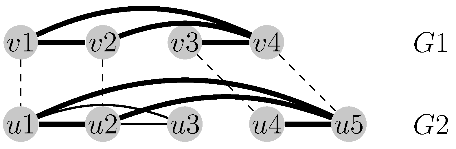
Figure 1.
Figure 1.
The alignment visualized with dashed lines maximizes the number of the common edges between the graphs and . The four activated common edges are emphasized in bold (i.e., ).
Figure 1.
The alignment visualized with dashed lines maximizes the number of the common edges between the graphs and . The four activated common edges are emphasized in bold (i.e., ).
Computing
is NP-hard following from [
18]. Nevertheless, maximum contact map overlap has been shown to be a meaningful way for comparing two protein structures [
5,
6,
7,
8,
9,
10,
11]. Previously, several distances have been proposed based on the maximum contact map overlap, for example
[
5,
7] and
[
6,
8,
11] with:
Note that and have been normalized, so that their values are in the interval and are, thus, measures of similarity between proteins. However, they are not metrics, as the next lemma shows.
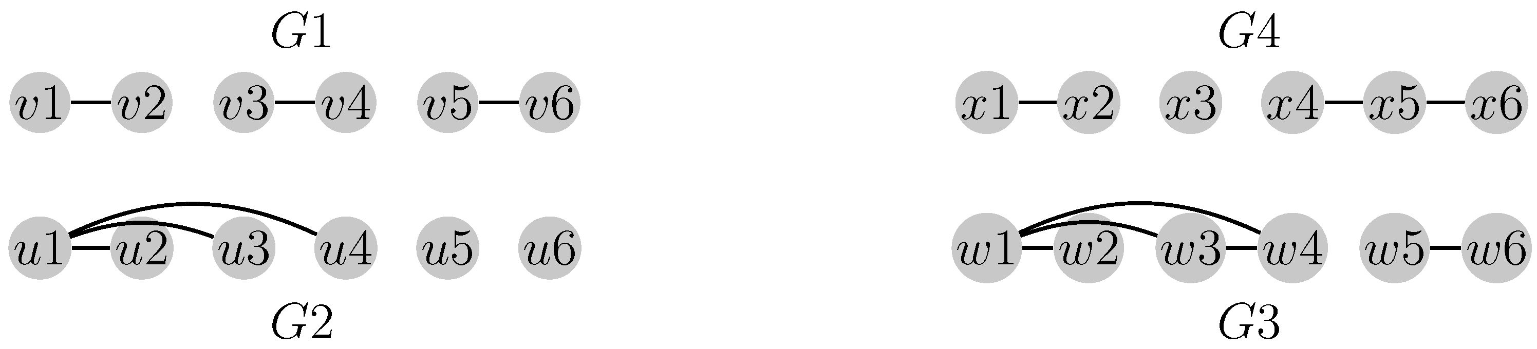
Lemma 1. Distances and do not satisfy the triangle inequality.
Proof. Consider the contact map graphs
in
Figure 2. It is easily seen that
and
. We then obtain:
Furthermore,
and
. We then obtain:
and:
as well as:
Figure 2.
Four contact map graphs.
Figure 2.
Four contact map graphs.
Let
be two contact map graphs. We propose a new similarity measure:
The following claim states that is a distance (metric) on the space of contact maps, and we refer to it as the max-CMO metric.
Lemma 2. is a metric on the space of contact maps.
Proof. To prove the triangle inequality for the function
, we consider three contact maps
, and we want to prove that
. We will use the fact that a similar function
on sets is a metric [
19], which is defined as:
The mapping
corresponding to
generates an alignment
, where
and
are ordered sets of vertices preserving the order of
V and
U, correspondingly. Since
is a one-to-one mapping, we can rename the vertices of
to the names of the corresponding vertices of
and keep the old names of the vertices of
. Denote the resulting ordered vertex set by
, and denote by
the corresponding set of edges. Define the graph
. Note that
and any common edge discovered by
has the same endpoints (after renaming) in
as in
; hence,
. Then, from Equation (
2):
Similarly, we compute the mapping corresponding to
and generate an optimal alignment
. As before, we use the mapping to rename the vertices of
to the corresponding vertices of
and denote the resulting sets of vertices and edges by
and
. Similarly to the above case, it follows that
. Combining the last two equalities, we get:
On the other hand,
contains only edges jointly activated by the alignments
and
, and its cardinality is not larger than
, which corresponds to the optimal alignment between
and
. Hence:
and, since
:
Combining the last inequality with Equation (
3) proves the triangle inequality for
. The other two properties of a metric, that
with equality if and only if
and
, are obviously also true. ☐
If instead of
, one computes lower or upper bounds for its value, replacing those values in Equation (
1) produces an upper or lower bound for
, respectively.
3. Nearest Neighbor Classification of Protein Structures
We suggest to approach the problem of classifying a given query protein structure with respect to a database of target structures based on a majority vote of the
k-nearest neighbors in the database. Nearest neighbor classification is a simple and popular machine learning strategy with strong consistency results; see, for example, [
20].
An important feature of our approach is that it is based on a metric, and we fully profit from all usual benefits when exploiting the structure introduced by that metric. In addition, we also model each protein family in the database as a ball with a specially-chosen protein from the family as the center, see
Section 3.1 for details. This allows one to obtain upper and lower bounds for the max-CMO distance in
Section 3.2, which are used to define a new dominance rule we call triangle dominance that proves to be very efficient. Finally, we describe in
Section 3.3 how these results can be used in a classification algorithm.
3.1. Finding Family Representatives
In order to minimize the number of targets with which a query has to be compared directly,
i.e., via computing an alignment, we designate a representative central structure for each family. Let
d denote any metric. Each family
can then be characterized by a representative structure
and a family radius
determined by:
In order to find and , we compute, during a preprocessing step, all pairwise distances within . We aim to compute these distances as precisely as possible, using a sufficiently long run time for each pairwise comparison. Since proteins from the same family are structurally similar, the alignment algorithm performs favorably, and we can usually compute intra-family distances optimally.
3.2. Dominance between Target Protein Structures
In order to find the target structures that are closest to a query q, we have to decide for a pair of Targets A and B which one is closer. We call such a relationship between two target structures dominance:
Lemma 3 (Dominance). Protein A dominates protein B with respect to a query q if and only if .
In order to conclude that A is closer to q than B, it may not be necessary to know and exactly. It is sufficient that A directly dominates B according to the following rule.
Lemma 4 (Direct dominance). Protein A dominates protein B with respect to a query q if , where and are an upper and lower bound on and , respectively.
Proof. It follows from the inequalities . ☐
Given a query
q, a target
A and the representative
of the family
of
A, the triangle inequality provides an upper bound, while the reverse triangle inequality provides respectively a lower bound on the distance from query
q to target
A:
We define the triangle upper (respectively lower) bound as:
Lemma 5.
Proof. ☐
Using Lemma 5, we derive supplementary sufficient conditions for dominance, which we call indirect dominance.
Lemma 6 (Indirect dominance). Protein A dominates protein B with respect to query q if .
Proof. . ☐
3.3. Classification Algorithm
k-nearest neighbor classification is a scheme that assigns the query to the class to which most of the
k targets belong that are closest to the query. In order to classify, we therefore need to determine the
k structures with minimum distance to the query and assign the superfamily to which the majority of the neighbors belong. As seen in the previous section, we can use bounds to decide whether a structure is closer to the query than another structure. This can be generalized to deciding whether or not a structure can be among the
k closest structures in the following way. We construct two priority queues, called LB and UB, whose elements are
and
, respectively, where
q is the query and
t is the target. Here,
(respectively
) is any lower (respectively upper) bound on the distance between
q and
t. In our current implementation, we use
as a distance, while lower and upper bounds are
(respectively
) or
(respectively
) where
and
are lower and upper bounds based on Lagrangian relaxation. As explained in [
8], these bounds can be polynomially computed by a sub-gradient descent method, where each iteration is solved in
time, where
n is the number of vertices of the contact map graph. However, when the graph is sparse (which is the case of contact map graphs), the above complexity bound is reduced to
. The practical convergence of the sub-gradient method is unpredictable, but an experimental analysis performed by the authors of [
8] suggests that 500 iterations is a reasonable average estimation. The quality of the bounds
and
for the purpose of protein classification has been already demonstrated in [
9,
11,
21].
The priority queues LB and UB are sorted in the order of increasing distance. The k-th element in queue UB is denoted by . Its distance to the query, , is the distance for which at least k target elements are closer to the query. Therefore, we can safely discard all of those targets that have a lower bound distance of more than to query q. That is, dominates all targets t for which .
We assume that distances between family members are computed optimally (this is actually done in our preprocessing step when computing the family representatives), i.e., if . The algorithm also works if this is not the case, then needs to be replaced by the corresponding Lagrangian bounds at the appropriate places.
4. Experimental Setup
We evaluated the classification performance and efficiency of different types of dominance of our algorithm on domains from SCOPCath [
22], a benchmark that consists of a consensus of the two major structural classifications SCOP [
1] (Version 1.75) and Cath [
2] (Version 3.2.0). We use this consensus benchmark in order to obtain a gold standard classification that very likely reflects structural similarities that are detectable automatically, since two classifications, each using a mix of expert knowledge and automatic methods, agree in their superfamily assignments. For generating SCOPCath, the intersection of SCOP and Cath has been filtered, such that SCOPCath only contains proteins with less than 50% sequence identity. Since this results in a rather small benchmark with only 6759 structures, we added these filtered structures for our evaluation in order to have a much larger, extended version of the benchmark, which is representative of the overlap between the existing classifications SCOP and Cath. There were 264 domains in extended SCOPCath that share more than 50% sequence similarity with a domain in SCOPCath, but do not both belong to the same SCOP family; since their families are perhaps not in SCOPCath and their classification in SCOP and Cath may not agree, we removed them. This way, we obtained
additional structures (
i.e., the extended benchmark is composed of
structures). These belong to 1348 superfamilies and 2480 families, of which 2093 families have more than one member. For SCOPCath, there are 1156 multi-member families. Structures and families are divided into classes according to
Table 1. For superfamily assignment, we compared a structure only to structures of the corresponding class, since class membership can in most cases be determined automatically, for example by a program that computes secondary structure content. In rare cases where class membership is unclear, one could combine the target structures of possible classes before classification. The four major protein classes are labeled from a to d and refer to: (a) all
α proteins,
i.e., consisting of
α-helices; (b) all
β proteins,
i.e., consisting of
β-sheets; (c)
α and
β proteins with parallel
β sheets,
i.e.,
β-
α-
β units; and (d)
α and
β proteins with antiparallel
β sheets,
i.e., segregated
α and
β regions. These classes are thus defined by secondary structure content and arrangement, which, in turn, is defined by class-specific contact map patterns. We therefore consider them individually when characterizing our max-CMO metric.
Table 1.
For every protein class, the table lists the number of structures in SCOPCath (str) and extended SCOPCath (ext), the corresponding number of families (fam) and superfamilies (sup).
Table 1.
For every protein class, the table lists the number of structures in SCOPCath (str) and extended SCOPCath (ext), the corresponding number of families (fam) and superfamilies (sup).
| Class | a | b | c | d | e | f | g | h | i | j | k |
|---|
| # str | 1195 | 1593 | 1774 | 1591 | 30 | 103 | 342 | 72 | 11 | 38 | 10 |
| # ext | 10,796 | 19,215 | 17,497 | 15,679 | 349 | 1006 | 2398 | 520 | 43 | 81 | 25 |
| # fam | 524 | 516 | 548 | 632 | 6 | 59 | 121 | 32 | 5 | 29 | 8 |
| # sup | 303 | 266 | 191 | 375 | 6 | 52 | 82 | 31 | 5 | 29 | 8 |
For classification, we randomly selected one query from every family with at least six members. This resulted in 236 queries for SCOPCath and 1369 queries for the extended SCOPCath benchmark.
We then computed all-
versus-all distances, Equation (
1), or distance bounds within each family using optimal maximum contact map overlap or the Lagrangian bound on it. For obtaining the latter, we use our Lagrangian solver A_purva [
8] (see also
https://www.irisa.fr/symbiose/software, as well as
http://csa.project.cwi.nl/), which reads PDB files, constructs contact maps and returns (bounds on) the contact map overlap. Using corresponding distance bounds, we determined the family representative according to Equation (
4). The complexity of this step is
, where
denotes the number of the members of the family
. Note that this step is query independent and is performed as a preprocessing. For every pairwise distance computation, we used a maximum time limit of 10 s. Since most comparisons were computed optimally, the average run time is approximately 2 s.
For every query, the nearest neighbor structures from SCOPCath and extended SCOPCath, respectively, were computed using our k-NN Algorithm 1. The algorithm is a two-step procedure. First, it improves bounds by applying several rounds of triangle dominance, for which the alignment from query to representatives is computed, and second, it switches to pairwise dominance, for which the alignment to any remaining target is computed. In the first step, query representative alignments are computed using an initial time limit of s; then, triangle dominance is applied to all targets, and the algorithm iterates with the time limit doubled until a termination criterion is met. This way, bounds on query target distances are improved successively. Since the query is compared uniquely with the family representative, only alignments are needed at each iteration. The computation of triangle dominance terminates if any of the following holds: (i) k targets are left; (ii) all query-representative distances have been computed optimally or with a time limit of 32 CPU seconds; (iii) the number of targets did not reduce from one round to the next. Pairwise dominance terminates if any of the following holds: (i) k targets are left; (ii) all remaining targets belong to the same superfamily; (iii) all query-target distances have been computed with a time limit of 32 CPU seconds. The query is then assigned to the superfamily to which the majority of the k-nearest neighbors belongs. In cases in which the pairwise dominance terminates with more than k targets or more than one superfamily remains, the exact k-nearest neighbors are not known. In that case, we order the targets based on the upper bound distance to the query and assign the superfamily using the top ten queries. In the case that there is a tie among the superfamilies to which the top ten targets belong, we report this situation.
We compare our exact
k-NN classifier with respect to classification accuracy with
k-NN classification using TM-align [
17] (Version 20130511). TM-align is a widely-used, fast structure alignment heuristic, which the authors, amongst others, applied for fold classification. TM-align alignments further were shown to have high accuracy with respect to manually-curated reference alignments [
23,
24]. Using TM-align, we align each query to all targets of the same class and compute the corresponding TM-score. The targets are then ranked based on TM-score (normalized with respect to query), and the superfamily that most of the
k nearest neighbors belong to is assigned.
In order to investigate the impact of k on classification accuracy, we additionally decreased k from nine to one, using each time the nearest neighbors from the classification result for . In the case that for a query, more than targets remained in this classification, we used all of them for searching for the k-nearest neighbors, but put an additional termination criterion if the number of structures after two or more iterations of pairwise dominance exceeds a given number. This effects only about a dozen queries that needed an extremely long run time for . If this termination criterion is applied, we do not obtain an exact classification, but shorter run times.
| Algorithm 1 Solving the k-NN classification problem |
- 1:
q // Query structure. - 2:
// Set of target structures. - 3:
// Family representatives; see Equation (4).- 4:
for all families // Distance from all family members to the respective representative. - 5:
, // Bounds on the distance from the query to the family representatives. - 6:
LB // Priority queue, which will hold the targets t in the order of increasing lower bound distance to the query. - 7:
UB // Priority queue, which will hold the targets t in the order of increasing upper bound distance to the query. - 8:
// A pointer to the k-th element in UB - 9:
1 s // Time limit for pairwise alignment. - 10:
for do - 11:
FAM belongs to family // Number of family members. - 12:
end for - 13:
while and changes do - 14:
2 - 15:
for with FAM do - 16:
Recompute and using time limit τ - 17:
for do - 18:
Update priority of t in LB to . // Bound from inverse triangle inequality Equation (7).- 19:
Update priority of t in UB to . // Bound from triangle inequality Equation (6).- 20:
end for - 21:
end for - 22:
// Check for targets dominated by . - 23:
for target t in do - 24:
if then - 25:
- 26:
LB ← LB - 27:
UB ← UB - 28:
FAM FAM where is the family of t. - 29:
end if - 30:
end for - 31:
if then - 32:
return The majority superfamily membership among . - 33:
end if - 34:
end while - 35:
Apply the dominance protocol for query q and targets as described in [ 9]. (The quality of the bounds and are improved by stepwise incrementing τ within the given time limit. At each step, the direct dominance (Lemma (4)) is applied for the targets from the updated .)
|
5. Computational Results
5.1. Characterizing the Distance Measure
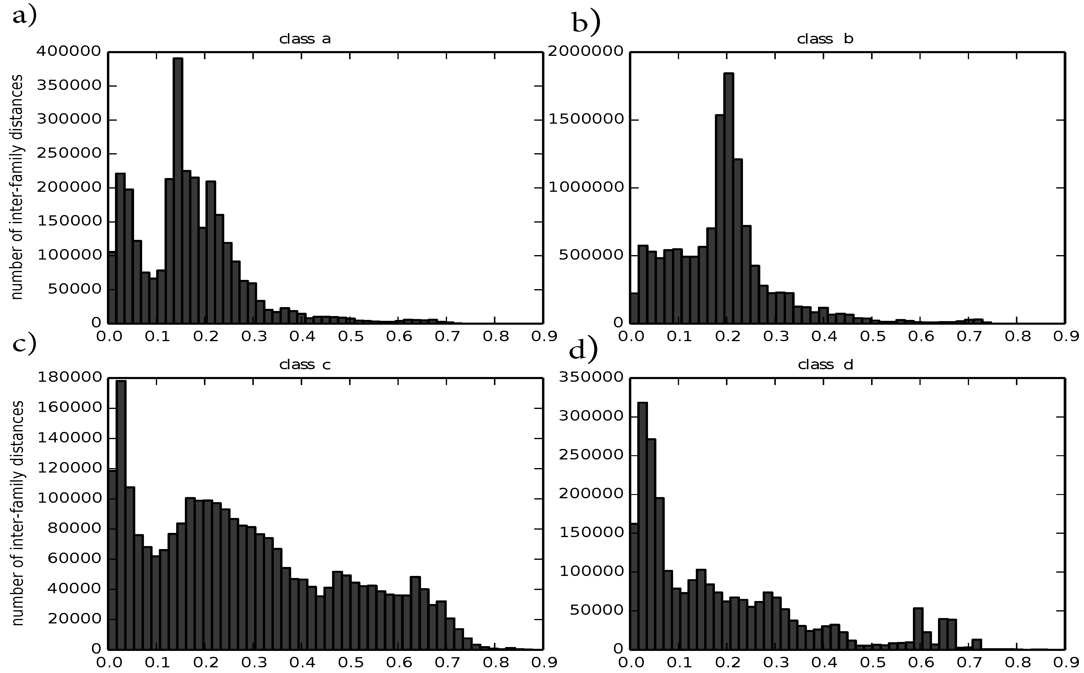
In the first preprocessing step, we evaluate how well our distance metric captures known similarities and differences between protein structures by computing intra-family and inter-family distances. A good distance for structure comparison should pool similar structures,
i.e., from the same family, whereas it should locate dissimilar structures from different families far apart from each other. In order to quantify such characteristics, we compute for each family with at least two members a central, representative structure according to Equation (
4). Therefore, we compute the distance between any two structures that belong to the same family. Such intra-family distances should ideally be small. We observe that the distribution of intra-family distances differ between classes and are usually smaller than 0.5, except for class c. For the four major protein classes a to d, there is a distance peak close to zero and another one around 0.2. For the four major protein classes, they are visualized in
Figure 3.
Figure 3.
Histograms of intra-family distances divided by class: (a) corresponds to class a; (b) corresponds to class b; (c) corresponds to class c; (d) corresponds to class d.
Figure 3.
Histograms of intra-family distances divided by class: (a) corresponds to class a; (b) corresponds to class b; (c) corresponds to class c; (d) corresponds to class d.
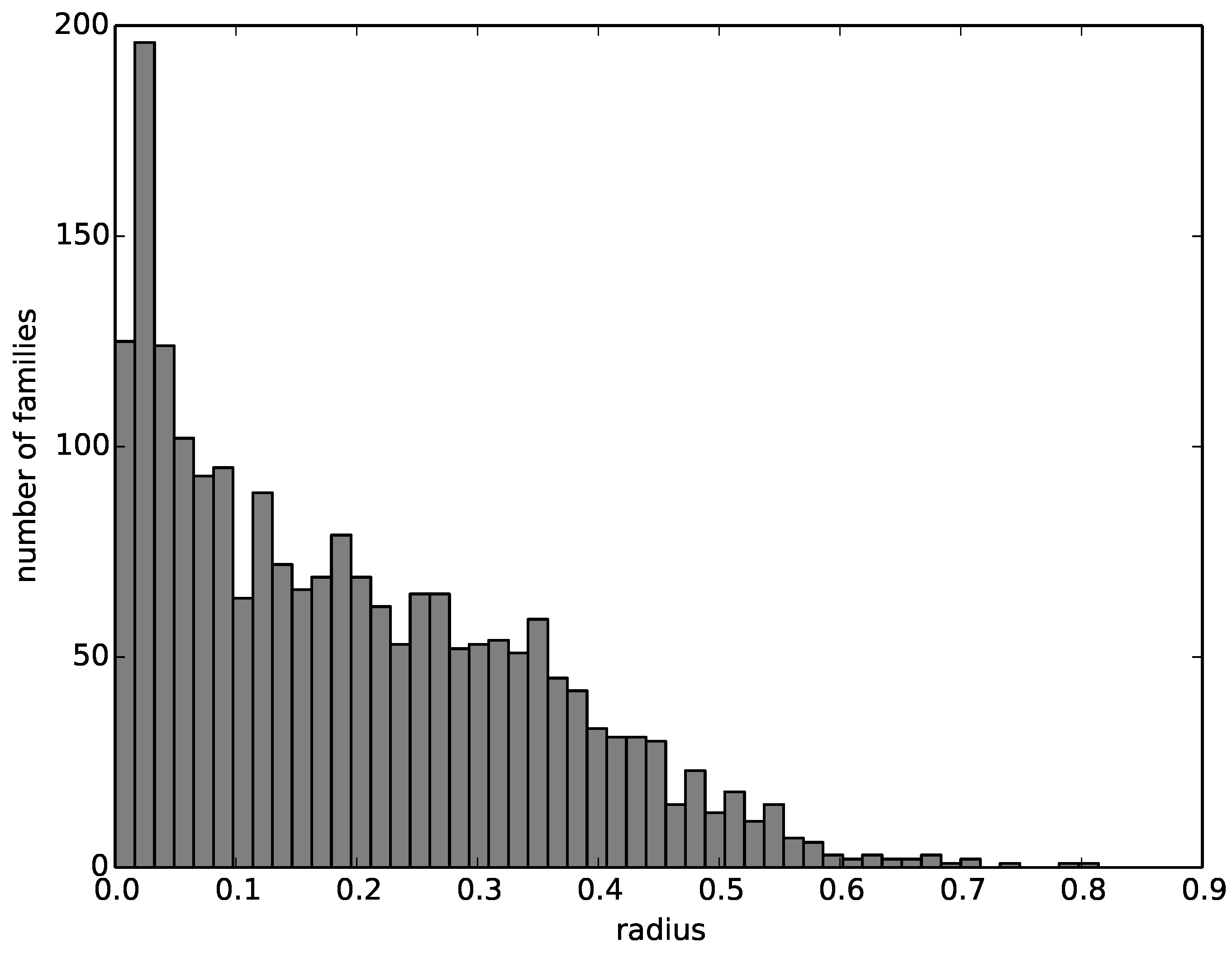
We then compute a radius around the representative structure that encompasses all structures of the corresponding family. The number of families with a given radius decreases nearly linearly from zero to 0.6, with most families having a radius close to zero and almost no families having a radius greater than 0.6. The histogram of family radii is visualized in
Figure 4.
Figure 4.
A histogram of the radii of the multi-member families.
Figure 4.
A histogram of the radii of the multi-member families.
Figure 5.
Histograms of overlap values between any two multi-member families for the four main classes a–d: (a) corresponds to class a; (b) corresponds to class b; (c) corresponds to class c; (d) corresponds to class d. The title gives an interval on the percentage of overlapping families, computed by using lower and upper bounds, respectively.
Considering that the distance metric is bound to be within zero and one, intra-family distances and radii show that the distance overall captures the similarity between structures well. Further, we investigate the distance between protein families by computing their overlap value as defined by
; for a histogram, see
Figure 5. Most families are not close to each other according to our distance metric. Families of the four most populated classes, which belong to different superfamilies, overlap in 23% to 25% of cases for class a, 11% to 18% for class b, 10% to 22% for class c and 11% to 18% for class d. These bounds on the number of overlapping families can be obtained by using the lower and upper bounds on the distances between representatives and the distances between family members appropriately.
5.2. Results for SCOPCath Benchmark
When classifying the 236 queries of SCOPCath, we achieve between 89% and 95% correct superfamily assignments; see
Table 2. Remarkably, the highest accuracy is reached for
k = 1, so here, just classifying the query as belonging to the superfamily of the nearest neighbor is the best choice. Our
k-NN classification resulted for any
k in a large number of ties, especially for
k = 2; see
Table 2. These currently unresolved ties also decrease assignment accuracy compared to
, for which a tie is not possible.
Table 2 further lists the number of queries that have been assigned, where exact denotes that the provable
k nearest neighbors have been computed. The percentage of exactly-computed nearest neighbors varies between 50% and 99% and increases with decreasing
k. A likely reason for this is that the larger the
k, the weaker is the
k-th distance upper bound that is used for domination, especially if the target on rank
k is dissimilar to the query. Since SCOPCath domains have low sequence similarity, this is likely to happen. It is also interesting to note that there are for any
k quite a few queries that have been assigned exactly, but that are nonetheless wrongly assigned; see
Table 2. These are cases in which our distance metric fails in ranking the targets correctly with respect to the gold standard.
Table 2.
Classification results showing the number of queries out of the overall 236 queries that have been assigned to a superfamily, the number of correct assignments, the number of assignments computed exactly, thereof the number of correct classifications and the number of ties that do not allow a superfamily assignment based on majority vote. The last two lines display the number of correct assignments and ties for k-NN classification using TM-align.
| k | 10 | 9 | 8 | 7 | 6 | 5 | 4 | 3 | 2 | 1 |
|---|
| # correct | 210 | 211 | 213 | 213 | 214 | 217 | 217 | 219 | 213 | 224 |
| # exact | 117 | 143 | 156 | 165 | 188 | 206 | 204 | 211 | 209 | 234 |
| # exact and correct | 110 | 134 | 149 | 155 | 178 | 198 | 195 | 205 | 206 | 224 |
| # ties | 10 | 9 | 11 | 8 | 10 | 10 | 10 | 10 | 20 | 0 |
| # TM-align correct | 219 | 220 | 220 | 225 | 225 | 228 | 226 | 227 | 226 | 228 |
| # TM-align ties | 4 | 4 | 9 | 5 | 5 | 3 | 8 | 5 | 8 | 0 |
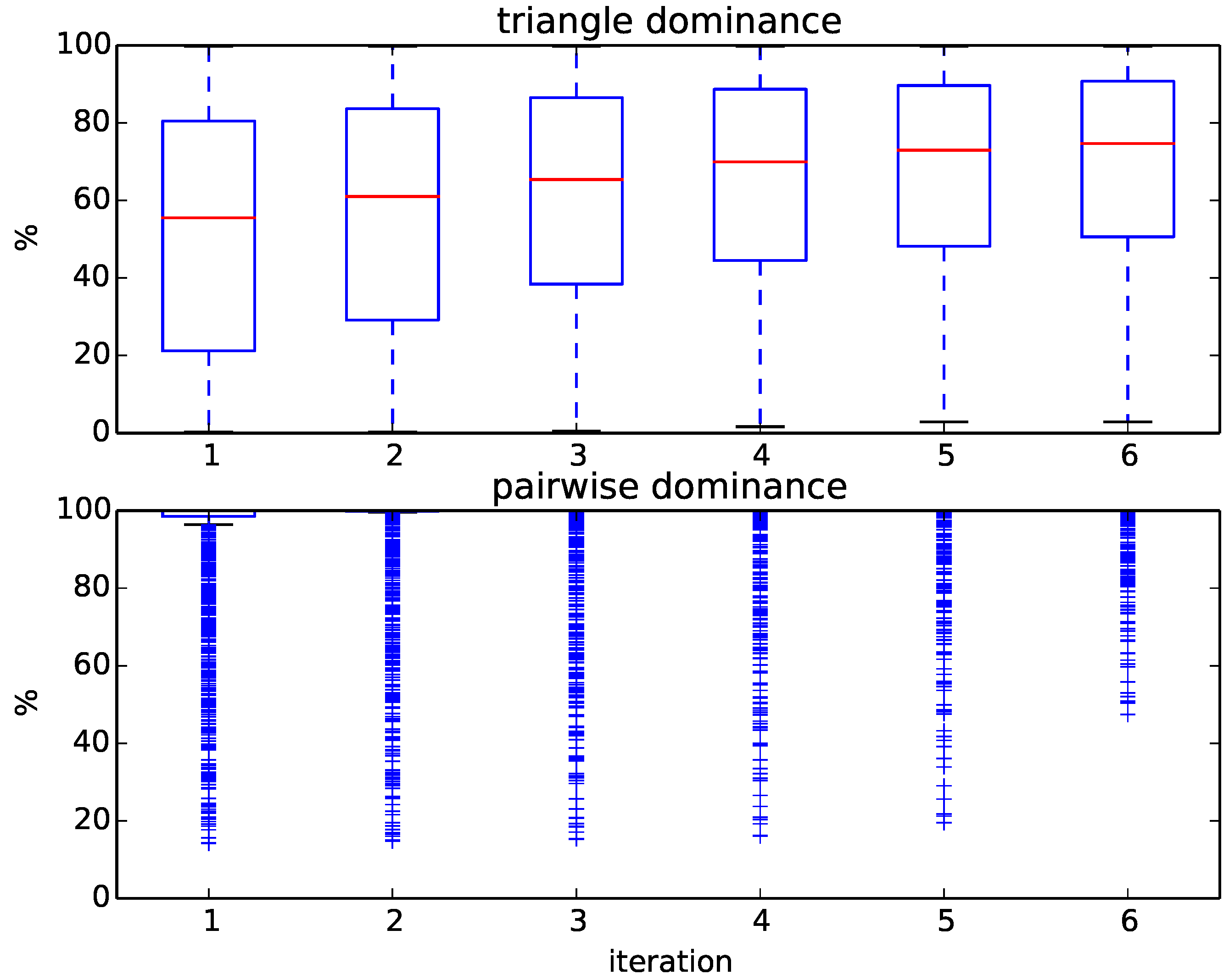
Figure 6 displays the progress of our algorithm in terms of the percentages of removed targets. We initially compute six rounds of triangle dominance, starting with one CPU second for every query representative alignment and doubling the run time every iteration up to 32 CPU seconds. The same is done in the pairwise dominance step of the algorithm, in which we compute the distance from the query to every remaining target. As shown in
Figure 6, the percentage of dominated targets within each iteration varies widely between queries, which results in a large variance of run times between queries. For some queries, up to 80% of targets can be removed by just computing the distance to the family representatives using a time limit of 1 s and applying triangle dominance; for others, even after several iterations of pairwise dominance, 50% of targets remain. Overall, most queries need, after triangle dominance, several iterations of pairwise dominance before being assigned, and quite a few cannot even be assigned exactly.
Figure 6.
Boxplots of the percentage of removed targets at each iteration during triangle and pairwise dominance for the 236 queries of the SCOPCath benchmark.
Figure 6.
Boxplots of the percentage of removed targets at each iteration during triangle and pairwise dominance for the 236 queries of the SCOPCath benchmark.
5.3. Results for Extended SCOPCath Benchmark
Our exact
k-NN classification can also be successfully applied to larger benchmarks, like extended SCOPCath, which are more representative of databases, such as SCOP. Here, the benefit of using a metric distance, triangle inequality and
k-NN classification is more pronounced. Remarkably, our classification run time on this benchmark that is about an order of magnitude larger than SCOPCath is for most queries of the same order of magnitude as run times on SCOPCath (except for some queries that need an extremely long run time and finally cannot be assigned exactly). Furthermore, here, run time varies extremely between queries, between
and
h for queries of the four major classes that could be assigned exactly. The median run time for all 1120 exactly assigned extended SCOPCath queries is
h. The classification results for extended SCOPCath are shown in
Table 3. Slightly more queries have been assigned correctly compared to SCOPCath, and significantly more queries have been assigned exactly. Both may reflect that there are now more similar structures within the targets. Further, the number of ties is decreased.
Table 3.
Classification results showing the number of queries out of the overall 1369 queries that have been assigned to a superfamily, the number of correct assignments, the number of assignments computed exactly, thereof the number of correct classifications and the number of ties that do not allow a superfamily assignment based on majority vote. The last two lines display the number of correct assignments and ties for k-NN classification using TM-align.
| k | 10 | 9 | 8 | 7 | 6 | 5 | 4 | 3 | 2 | 1 |
|---|
| # correct | 1303 | 1331 | 1334 | 1341 | 1341 | 1346 | 1344 | 1351 | 1348 | 1361 |
| # exact | 1120 | 1182 | 1228 | 1271 | 1286 | 1339 | 1341 | 1352 | 1347 | 1368 |
| # exact and correct | 1104 | 1166 | 1215 | 1257 | 1276 | 1329 | 1330 | 1341 | 1343 | 1360 |
| # ties | 35 | 5 | 12 | 6 | 11 | 7 | 9 | 3 | 17 | 0 |
| # TM-align correct | 1311 | 1347 | 1346 | 1350 | 1351 | 1354 | 1352 | 1353 | 1351 | 1361 |
| # TM-align ties | 39 | 4 | 7 | 4 | 6 | 4 | 4 | 5 | 15 | 0 |
Figure 7 displays the progress of the computation. Here, many more target structures are removed by triangle dominance and within the very first iteration of pairwise dominance compared to the SCOPCath benchmark. For example, for most queries, more than 60% of targets are removed by triangle dominance alone. Only very few queries need to explicitly compute the distance to a large percentage of the targets, and almost 75% of queries can be assigned after only one round of pairwise dominance.
Figure 7.
Boxplots of the percentage of removed targets at each iteration during triangle and pairwise dominance for the 1369 queries of the extended SCOPCath benchmark.
Figure 7.
Boxplots of the percentage of removed targets at each iteration during triangle and pairwise dominance for the 1369 queries of the extended SCOPCath benchmark.
6. Discussion
The difficulty to optimally compute a superfamily assignment using k-NN increases with the dissimilarity of the k-th closest target and the query, because this target determines the domination bound, and this bound becomes weaker when k increases. This can be observed in the different number of exactly-assigned queries between SCOPCath and extended SCOPCath, on the one hand, and for different k, on the other hand. Since SCOPCath has been filtered for low sequence identity, we can expect that the k-th neighbor is less similar to the query than the k-th neighbor in extended SCOPCath, and therefore, it is easier to compute extended SCOPCath exactly. Accordingly, the number of exactly-assigned queries tends to increase with decreasing k. In future work, we may use such properties of the distance bounds to decide which k is most appropriate for a given query.
Our exact classification is based on a well-known property of exact CMO computation: similar structures are quick to align and are usually computed exactly, whereas dissimilar structures are extremely slow to align and usually not exactly. Therefore, we remove dissimilar structures early using bounds. Distances between similar structures can then be computed (near-)optimal, and the resulting k-NN classification is exact.
Except for the case on the extended benchmark, in terms of assignment accuracy, TM-align performs slightly better than max-CMO, and it usually has to some extent fewer ties. On the other hand, both max-CMO and TM-align perform best in the case , and for that most relevant case, the two methods have the same accuracy. Considering that max-CMO is a metric and, thus, needs to compare structures globally, while TM-align is not, it still allows one to perform very accurate superfamily assignment.
While for the extended benchmark, max-CMO and TM-align have the same number of correct classifications for the best choice of value for k, the somewhat better performance of TM-align in the other cases indicates that the max-CMO method could be further improved. A possible disadvantage of our metric is that it does not apply proper length normalization. For instance, if a protein structure is identical to a substructure of another protein, the corresponding max-CMO distance depends on the length of the longer protein. For classification purposes, it would usually be better to rank a protein with such local similarity higher than another protein that is less similar, but of smaller length.
Moreover, although the current results suggest that, in terms of assignment accuracy, using only the nearest neighbor for classification works best, finding the k-nearest neighbor structures is still interesting and important. A new query structure is in need of being characterized, and the set of k closest structures from a given classification gives a useful description on its location in structure space, especially if this space is metric. Note that, besides using the presented algorithm for determining the k-nearest neighbors, it could straightforwardly also be used to find all structures within a certain distance threshold of a given query.
We show that our approach is beneficial for handling large datasets, the structures of which form clusters in some metric space, because it can quickly discard dissimilar structures using metric properties, such as triangle inequality. This way, the target dataset does not need to be reduced previously using a different distance measure, such as sequence similarity, which can lead to mistakes. Our classification is at all times based exclusively on structural distance.
Among the disadvantages of a heuristic approach for the task of large-scale structure classification, we can point to the observation that the obtained classifications are not stable. As versions of tools or random seeds change, the distance between structures may change, since the provable distance between two structures is not known. With these distance changes, also the entire classification may change. Such possible, unpredictable changes in classification contradict the essential use of an automatic classification as a reference. Furthermore, even if a given heuristic could be very fast, it always requires a pairwise number of comparisons for solving the classification problem by the k-NN approach. This requirement obviously becomes a notable hindrance with the natural and quick increase of the protein databases size.
7. Conclusion
In this work, we introduced a new distance based on the CMO measure and proved that it is a true metric, which we call the max-CMO metric. We analyzed the potential of max-CMO for solving the k-NN problem efficiently and exactly and built on that basis a protein superfamily classification algorithm. Depending on the values of k, our accuracy varies between 89% for and 95% for for SCOPCath and between 95% and 99% for extended SCOPCath. The fact that the accuracy is highest for indicates that using more sophisticated rules than k-NN may produce even better results.
In summary, our approach provides a general solution to k-NN classification based on a computationally-intractable measure for which upper and lower bounds are polynomially available. By its application to a gold standard protein structure classification benchmark, we demonstrate that it can successfully be applied for fully-automatic and reliable large-scale protein superfamily classification. One of the biggest advantages of our approach is that it permits one to describe the protein space in terms of clusters with their representative central structures, radii, intra-cluster and inter-clusters distances. Such a formal description is by itself a source of knowledge and a base for future analysis.


 ,
, 


